Inference Algorithms

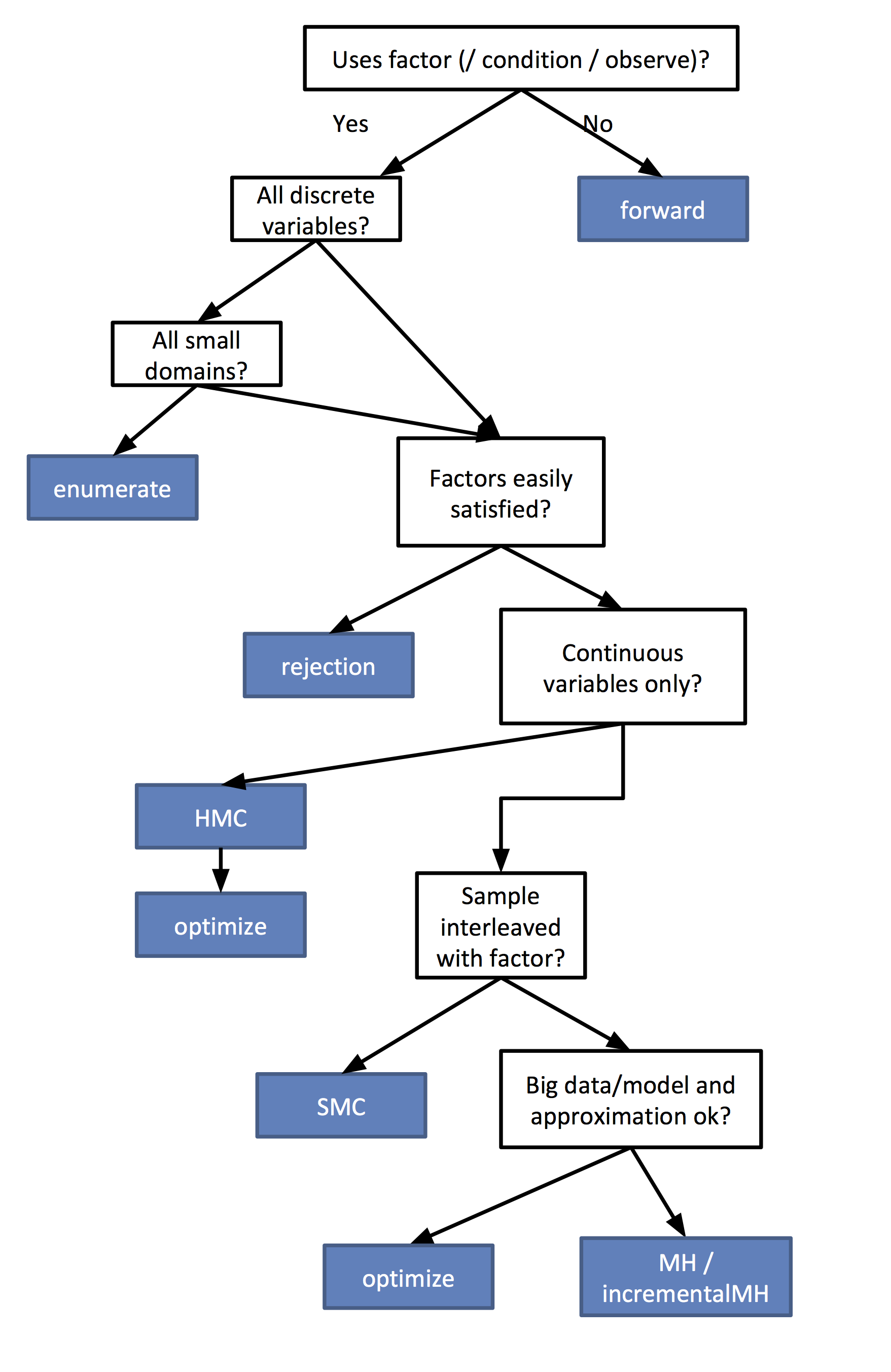
Flow chart for determining your best inference algorithm

drawing

Enumeration

Enumeration essentially “does the math”. It builds a big tree of all the possible outcomes and their associated probabilities. It only works if you have ONLY discrete variables, and the more variables you have, the longer it takes.

var model = function(){
	var x = uniformDraw(_.range(0, 10))
	var y = uniformDraw(_.range(0, 10))
	condition(x + y > 10)
	return {x, y}
}

var posterior = Infer({model, method: "enumerate"})
viz(posterior)

Rejection sampling

Rejection sampling randomly samples values for all the random variables, check to see if the condition is true, and if it is false, it tries again. Rejection can also work with “soft conditions” (aka factors). The more improbable the condition statement is, the longer it takes to run.

var model = function(){
	var x = uniform(0, 10)
	var y = uniform(0, 10)
	condition(x + y > 10)
	return {x, y}
}

var posterior = Infer({model, method: "rejection", samples: 1000})
viz(posterior)

MCMC (aka Single-site Metropolis-Hastings)

MCMC in WebPPL is a single-site Metropolis Hastings algorithm. It starts by randomly sampling values for all of the variables. Then, it randomly picks one of the variables and resamples its value; before re-running the program, it checks the Metropolis-Hastings (MH) recipe… if MH says it is a good idea, it accepts the new value, and re-runs the program. If MH indicates it’s a bad new value of the variable, it rejects the proposal, and tries to resample a different value.

The run-time of MH scales with the number of iterations, a pre-defined value. However, the results are only gauranteed to represent the true posterior distribution in the limit. The difficulty in approximating the true posterior distribution will depend on details of the model and data. If you have correlated parameters (e.g., when your model is overparamaterized), MCMC-MH will have a hard time working.

var model = function(){
	var xs = repeat(10, function(){ uniform(0, 10) } )
	var ys = repeat(10, function(){ uniform(0, 10) } )
	map2(function(x, y){
		condition(x + y > 10)
	}, xs, ys)
	return xs
}

var posterior = Infer({model, method: "MCMC", 
                       samples: 1000, burn: 1000})
viz.marginals(posterior)

HMC

var model = function(){
	var xs = repeat(10, function(){ uniform(0, 10) } )
	var ys = repeat(10, function(){ uniform(0, 10) } )
	map2(function(x, y){
		factor(x + y)
	}, xs, ys)
	return xs
}

var posterior = Infer({model, method: "MCMC", 
                       kernel: {HMC: {steps: 5, stepSize: 0.05}}, 
                       samples: 1000, burn: 500})
viz.marginals(posterior)

Incremental MH

WebPPL includes a version of MCMC with local cacheing. This can be useful when doing Bayesian Data Analysis when you have participant- or item-wise parameters which only influence the part of the model that deals with that particular participant or item. It only re-runs the program for the part of the model that is affected by the variable.

var model = function(){

	var a = uniform(0, 10)

	map(function(i){
		var x = uniform(0, 10)
		var y = uniform(0, 10)
		condition( a * (x + y) > 10)
	}, _.range(0, 10))

	return a
}

var posterior = Infer({model, method: "incrementalMH", samples: 1000})
viz(posterior)

Forward

Forward is not really an inference algorithm so much as it is repeatedly sampling from the prior. One virtue of using the "forward" method is that it returns to you a distribution object.

Forward will ignore observe(), condition(), or factor() statements that may appear in the model.

var model = function(){

	var x = uniform(0, 10)
	var y = uniform(0, 10)
	return x + y 
}

var posterior = Infer({model, method: "forward", samples: 1000})
viz(posterior)

Others

In the next chapter, we will look at an example of doing Bayesian data analysis over a Bayesian cognitive model.

Table of Contents